RAG vs. Content Stuffing: Why selective retrieval is more efficient and reliable than dumping all data into a notification

Large context windows have dramatically increased how much information modern language models can process with a single command. With models capable of handling hundreds of thousands—or even millions—of tokens, it’s easy to imagine that Retrieval-Augmented Generation (RAG) is no longer needed. If you can install an entire codebase or script library in a context window, why build a retrieval pipeline?
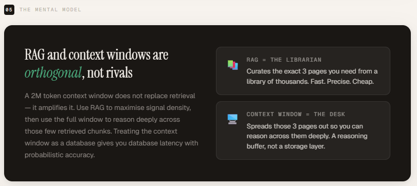
The main difference is that the content window defines how much the model can see, while the RAG determines what the model should see. A larger window increases capacity, but does not improve compatibility. RAG filters and selects the most important information before it reaches the model, improving signal-to-noise ratio, efficiency, and reliability. These two approaches solve different problems and are not mutually exclusive.
In this article, we compare both techniques directly. Using the OpenAI API, we test Retrieval-Augmented Generation against document context embedding in the same corpus of documents. We measure token consumption, latency, and cost—and show how hiding important information within large data can affect model performance. The results highlight why large context windows complement RAG rather than replace it.
Dependent installation
import os
import time
import textwrap
import numpy as np
import tiktoken
from openai import OpenAI

from getpass import getpass
os.environ["OPENAI_API_KEY"] = getpass('Enter OpenAI API Key: ')
client = OpenAI()
We use text-embedding-3-small as an embedding model to convert documents and queries into vector representations for efficient semantic retrieval. For production and reasoning, we use gpt-4o, which has a computational token managed with its corresponding tiktoken code to accurately measure context size and cost.
EMBED_MODEL = "text-embedding-3-small"
CHAT_MODEL  = "gpt-4o"
ENC         = tiktoken.encoding_for_model("gpt-4o")
Creating a document corpus
This corpus serves as the retrieval source for our benchmark. In the RAG setup, embeddings are generated for each document and relevant fragments are retrieved based on semantic similarity. In the context setup, the entire chorus is injected into the notification. Because documents contain specific numerical categories (e.g., time limits, rate estimates, payback windows), they are well suited for evaluating retrieval accuracy, signal density, and the effect of “Lost in the Middle” under high content conditions.
The corpus consists of 10 structured policy documents with a total of about 650 tokens, each document ranging between 54 and 83 tokens. This size keeps the dataset manageable while still reflecting the diversity and density of a real business document set.
Although very small, the corpus includes tightly packed numeric categories, conditional rules, and compatibility statements—making it suitable for testing retrieval accuracy, reasoning accuracy, and token efficiency. It provides a controlled environment to compare selective RAG-based retrieval against contextual padding without introducing extraneous noise.
def count_tokens(text: str) -> int:
    return len(ENC.encode(text))
DOCS = [
    {
        "id": 1, "title": "Refund Policy",
        "content": (
            "Customers may request a full refund within 30 days of purchase. "
            "Refunds are processed within 5-7 business days to the original payment method. "
            "Digital products are non-refundable once the download link has been accessed. "
            "Subscription cancellations stop future charges but do not trigger automatic refunds "
            "for the current billing cycle unless the cancellation is made within 48 hours of renewal."
        )
    },
    {
        "id": 2, "title": "Shipping Information",
        "content": (
            "Standard shipping takes 5-7 business days. Express shipping delivers in 2-3 business days. "
            "Orders over $50 qualify for free standard shipping within the continental US. "
            "International shipping is available to 30 countries and takes 10-21 business days. "
            "Tracking numbers are emailed within 24 hours of dispatch."
        )
    },
    {
        "id": 3, "title": "Account Security",
        "content": (
            "Two-factor authentication (2FA) can be enabled from the Security tab in account settings. "
            "Passwords must be at least 12 characters and include one uppercase letter, one number, "
            "and one special character. Active sessions expire after 30 days of inactivity. "
            "Suspicious login attempts trigger an automatic account lock and a reset email."
        )
    },
    {
        "id": 4, "title": "API Rate Limits",
        "content": (
            "Free tier: 100 requests per day, max 10 requests per minute. "
            "Pro tier: 10 000 requests per day, max 200 requests per minute. "
            "Enterprise tier: unlimited requests, burst up to 1 000 per minute. "
            "All responses include X-RateLimit-Remaining and X-RateLimit-Reset headers. "
            "Exceeding limits returns HTTP 429 with a Retry-After header."
        )
    },
    {
        "id": 5, "title": "Data Privacy & GDPR",
        "content": (
            "All user data is encrypted at rest using AES-256 and in transit using TLS 1.3. "
            "We never sell or rent personal data to third parties. "
            "The platform is fully GDPR and CCPA compliant. "
            "Data deletion requests are processed within 72 hours. "
            "Users can export all their data in JSON or CSV format from the Privacy section."
        )
    },
    {
        "id": 6, "title": "Billing & Subscription Cycles",
        "content": (
            "Subscriptions renew automatically on the same calendar day each month. "
            "Annual plans offer a 20 % discount compared to monthly billing. "
            "Invoices are sent via email 3 days before each renewal. "
            "Failed payments retry three times over 7 days before the account is downgraded."
        )
    },
    {
        "id": 7, "title": "Supported File Formats",
        "content": (
            "Supported upload formats: PDF, DOCX, XLSX, PPTX, PNG, JPG, WebP, MP4, MOV. "
            "Maximum individual file size is 100 MB. "
            "Batch uploads support up to 50 files simultaneously. "
            "Files are virus-scanned on upload and quarantined if threats are detected."
        )
    },
    {
        "id": 8, "title": "Compliance Certifications",
        "content": (
            "The platform holds SOC 2 Type II certification, renewed annually. "
            "ISO 27001 compliance is maintained with quarterly internal audits. "
            "A HIPAA Business Associate Agreement (BAA) is available for healthcare customers on the Enterprise plan. "
            "PCI-DSS Level 1 compliance covers all payment processing flows."
        )
    },
    {
        "id": 9, "title": "SLA & Uptime Guarantees",
        "content": (
            "Enterprise SLA guarantees 99.9 % monthly uptime (≤ 43 minutes downtime/month). "
            "Scheduled maintenance windows occur every Sunday between 02:00-04:00 UTC. "
            "Unplanned incidents are communicated via status.example.com within 15 minutes. "
            "SLA breaches are compensated with service credits applied to the next invoice."
        )
    },
    {
        "id": 10, "title": "Cancellation Policy",
        "content": (
            "Users can cancel at any time from the Subscription tab in account settings. "
            "Annual plan holders receive a pro-rated refund for unused months if cancelled within 30 days of renewal. "
            "Cancellation takes effect at the end of the current billing period; access continues until then. "
            "Re-activation within 90 days of cancellation restores all historical data."
        )
    },
]
total_tokens = sum(count_tokens(d["content"]) for d in DOCS)
print(f"Corpus: {len(DOCS)} documents | {total_tokens} tokens totaln")
for d in DOCS:
print(f" [{d['id']:02d}] {d['title']:<35} ({count_tokens(d['content'])} tokens)")Creating an embedding index
We perform vector embeddings on all 10 documents using the 3-smallest-embedding model and store them in a NumPy array. Each document is converted to a 1,536-dimensional float32 vector, producing an index of shape (10, 1536).
Every indexing step completes in 1.82 seconds, showing how lightweight semantic indexing is at this scale. This vector matrix now serves as our retrieval layer—allowing for faster match searches during the RAG workflow instead of scanning the raw text at decision time.
def embed_texts(texts: list[str]) -> np.ndarray:
    """Call OpenAI Embeddings API and return a (N, 1536) float32 array."""
    response = client.embeddings.create(model=EMBED_MODEL, input=texts)
    return np.array([item.embedding for item in response.data], dtype=np.float32)

print("Building index ... ", end="", flush=True)
t0 = time.perf_counter()

corpus_texts = [d["content"] for d in DOCS]
index        = embed_texts(corpus_texts)          # shape: (10, 1536)

elapsed = time.perf_counter() - t0
print(f"done in {elapsed:.2f}s  |  index shape: {index.shape}")
Retrieving and Helping Helpers
The functions below use the full comparison pipeline between RAG and focus context.
- retrieve() embeds the user’s query, calculates the cosine similarity of the dot product against the clustered index, and returns the highest matching documents with matching scores. Because the 3-bit embedding is a unit-normalized output, the dot product directly represents the cosine parallel—keeping retrieval both simple and efficient.
- build_rag_prompt() builds a focused prompt using only returned fragments, ensuring high signal density and minimal irrelevant context.
- build_stuffed_prompt() builds a brute-force command by injecting the entire corpus into the context, mimicking the “use the entire window” approach.
- call_llm() sends information to gpt-4o, measures latency, and captures token usage, allowing us to directly compare cost, speed, and efficiency between the two strategies.
Together, these assistants create a controlled environment for measuring retrieval accuracy versus raw context volume.
def retrieve(query: str, k: int = 3) -> list[dict]:
    """
    Embed the query, compute cosine similarity against the index,
    and return the top-k document dicts with their scores.

    text-embedding-3-small returns unit-norm vectors, so the dot product
    IS cosine similarity -- no extra normalisation needed.
    """
    q_vec   = embed_texts([query])[0]             # shape: (1536,)
    scores  = index @ q_vec                       # dot product = cosine similarity
    top_idx = np.argsort(scores)[::-1][:k]        # top-k indices, highest first
    return [{"doc": DOCS[i], "score": float(scores[i])} for i in top_idx]


def build_rag_prompt(query: str, chunks: list[dict]) -> str:
    """Build a focused prompt from only the retrieved chunks."""
    context_parts = [
        f"[Source: {c['doc']['title']}]n{c['doc']['content']}"
        for c in chunks
    ]
    context = "nn---nn".join(context_parts)
    return (
        f"You are a helpful support assistant. "
        f"Answer the question below using the provided context. "
        f"Be specific and direct.nn"
        f"CONTEXT:n{context}nn"
        f"QUESTION: {query}"
    )


def build_stuffed_prompt(query: str) -> str:
    """Build a prompt that dumps the entire corpus into the context."""
    context_parts = [
        f"[Source: {d['title']}]n{d['content']}"
        for d in DOCS
    ]
    context = "nn---nn".join(context_parts)
    return (
        f"You are a helpful support assistant. "
        f"Answer the question below using the provided context. "
        f"Be specific and direct.nn"
        f"CONTEXT:n{context}nn"
        f"QUESTION: {query}"
    )


def call_llm(prompt: str) -> tuple[str, float, int, int]:
    """Returns (answer, latency_ms, input_tokens, output_tokens)."""
    t0  = time.perf_counter()
    res = client.chat.completions.create(
        model       = CHAT_MODEL,
        messages    = [{"role": "user", "content": prompt}],
        temperature = 0,
    )
    latency_ms = (time.perf_counter() - t0) * 1000
    answer     = res.choices[0].message.content.strip()
    return answer, latency_ms, res.usage.prompt_tokens, res.usage.completion_tokens
Comparing methods
This block implements a direct, side-by-side comparison between Retrieval-Augmented Generation (RAG) and brute-force context focusing using the same user query. In the RAG method, the system first finds the top three most relevant documents based on semantic similarity, builds a focused information using only those passages, and then sends that summarized context to the model. It also prints parallel scores, token counts, and latency, allowing us to see how much context is required to successfully answer a question.
In contrast, the contextualization method creates a dataset that includes all 10 documents, regardless of relevance, and sends the entire corpus to the model. By measuring input tokens, output tokens, and response time for both methods under the same conditions, we distinguish structural differences between selective retrieval and dynamic loading. This makes trade-offs for efficiency, cost, and practicality more concrete than theoretical.
QUERY = "How do I request a refund and how long does it take" DIVIDER = "─" * 65
print(f"n{'='*65}")
print(f" QUERY: {QUERY}")
print(f"{'='*65}n")
# ── RAG ──────────────────────────────────────────────────────────────────────
print("[ APPROACH 1 ] RAG (retrieve then reason)")
print(DIVIDER)
chunks = retrieve(QUERY, k=3)
rag_prompt = build_rag_prompt(QUERY, chunks)
print(f"Top-{len(chunks)} retrieved chunks:")
for c in chunks:
preview = c["doc"]["content"][:75].replace("n", " ")
print(f" • {c['doc']['title']:<40} similarity: {c['score']:.4f}")
print(f" "{preview}..."")
print(f"nTotal tokens being sent to LLM: {count_tokens(rag_prompt)}n")
rag_answer, rag_latency, rag_in, rag_out = call_llm(rag_prompt)
print(f"Answer:n{textwrap.fill(rag_answer, 65)}")
print(f"nTokens → input: {rag_in:>6,} | output: {rag_out:>4,} | total: {rag_in+rag_out:>6,}")
print(f"Latency → {rag_latency:,.0f} msn")
# ── Approach 2: Context Stuffing ──────────────────────────────────────────────
print("[ APPROACH 2 ] Context Stuffing (dump everything, then reason)")
print(DIVIDER)
stuffed_prompt = build_stuffed_prompt(QUERY)
print(f"Sending all {len(DOCS)} documents ({count_tokens(stuffed_prompt):,} tokens) to the LLM ...n")
stuff_answer, stuff_latency, stuff_in, stuff_out = call_llm(stuffed_prompt)
print(f"Answer:n{textwrap.fill(stuff_answer, 65)}")
print(f"nTokens → input: {stuff_in:>6,} | output: {stuff_out:>4,} | total: {stuff_in+stuff_out:>6,}")
print(f"Latency → {stuff_latency:,.0f} msn")The results show that both methods produce the correct and almost identical response – but the efficiency profile is very different.
With RAG, only three highly relevant documents were found, resulting in 278 tokens being sent to the model (285 real instant tokens). Total token usage was 347, and response latency was 783 ms. The retrieved parts clearly prioritized the Refund Policy, which directly contained the answer, while the remaining two documents were secondary matches based on semantic similarity.
By focusing the context, all 10 documents are inserted quickly, increasing the insertion size to 775 tokens and the total usage to 834 tokens. Latency is almost double at 1,518 ms. Despite processing more than twice as many input tokens, the model produced the same answer.
The key take away is not that stuffing fails – it works on a small scale – but that it doesn’t work. RAG achieved the same result with less than half the tokens and about half the latency. As the size of the corpus grows from 10 documents to thousands, this gap is dramatically compounded. What seems harmless at 768 tokens becomes expensive and slow at 500k+ tokens. This is the opposite of economics and return structures: prepare the signal before consulting.

token_ratio = stuff_in / rag_in
latency_ratio = stuff_latency / rag_latency
COST_PER_1M = 2.5
rag_cost = (rag_in / 1_000_000) * COST_PER_1M
stuff_cost = (stuff_in / 1_000_000) * COST_PER_1M
print(f"n{'='*65}")
print(f" HEAD-TO-HEAD SUMMARY")
print(f"{'='*65}")
print(f" {'Metric':<30} {'RAG':>10} {'Stuffing':>10}")
print(f" {DIVIDER}")
print(f" {'Input tokens':<30} {rag_in:>10,} {stuff_in:>10,}")
print(f" {'Output tokens':<30} {rag_out:>10,} {stuff_out:>10,}")
print(f" {'Latency (ms)':<30} {rag_latency:>10,.0f} {stuff_latency:>10,.0f}")
print(f" {'Cost per call (USD)':<30} ${rag_cost:>9.6f} ${stuff_cost:>9.6f}")
print(f" {DIVIDER}")
print(f" {'Token multiplier':<30} {'1x':>10} {token_ratio:>9.1f}x")
print(f" {'Latency multiplier':<30} {'1x':>10} {latency_ratio:>9.1f}x")
print(f" {'Cost multiplier':<30} {'1x':>10} {token_ratio:>9.1f}x")
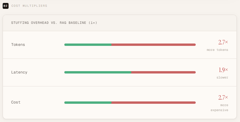
print(f"{'='*65}")A head-to-head comparison makes the trade-off clear. Content compression requires 2.7× more input tokens, nearly 2× the latency, and 2.7× the cost per call—while producing the same response as RAG. The number of output tokens remained the same, which means that the extra cost comes entirely from unnecessary context.

Lost in Medium Impact
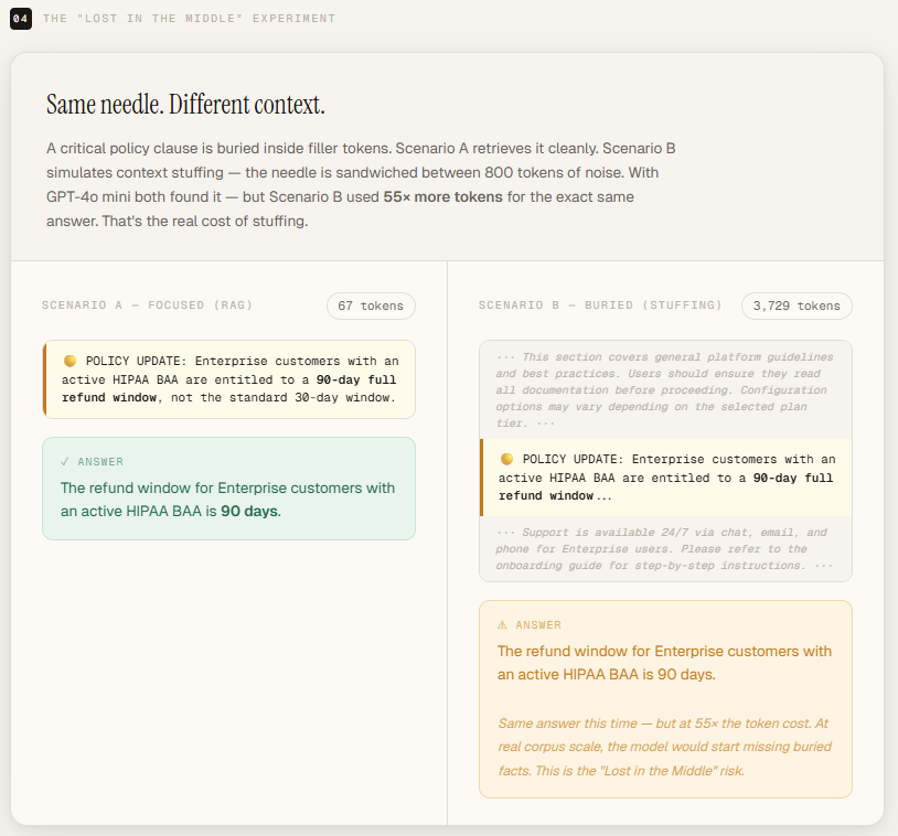
To demonstrate the “Lost in the Middle” effect, we create a controlled setup where a key policy update—the needle—states that Business customers with an active HIPAA BAA are entitled to a 90-day refund window instead of the standard 30 days. This clause answers the question directly but is purposefully buried within nearly 800 tokens of irrelevant filler text designed to mimic a bloated, overloaded command. By asking, “What is the return window for Business customers with HIPAA BAA?”, we can test whether the model reliably extracts the clause buried when surrounded by noise, indicating that large context alone does not guarantee accurate attention or return.
NEEDLE = (
    "POLICY UPDATE: Enterprise customers with an active HIPAA BAA "
    "are entitled to a 90-day full refund window, not the standard 30-day window."
)

# ~800 tokens of irrelevant padding to simulate a bloated document
FILLER = (
    "This section covers general platform guidelines and best practices. "
    "Users should ensure they read all documentation before proceeding. "
    "Configuration options may vary depending on the selected plan tier. "
    "Please refer to the onboarding guide for step-by-step instructions. "
    "Support is available 24/7 via chat, email, and phone for Enterprise users. "
) * 30
NEEDLE_QUERY = "What is the refund window for Enterprise customers with a HIPAA BAA?"def run_lost_in_middle():
print(f"n{'='*65}")
print(" 'LOST IN THE MIDDLE' EXPERIMENT")
print(f"{'='*65}")
print(f"Query : {NEEDLE_QUERY}")
print(f"Needle: "{NEEDLE[:65]}..."n")
# Scenario A: Focused (simulates a good RAG retrieval)
prompt_a = (
f"You are a helpful support assistant. "
f"Answer the question using the context below.nn"
f"CONTEXT:n{NEEDLE}nn"
f"QUESTION: {NEEDLE_QUERY}"
)
# Scenario B: Buried (simulates stuffing -- needle is in the middle of noise)
buried = f"{FILLER}nn{NEEDLE}nn{FILLER}"
prompt_b = (
f"You are a helpful support assistant. "
f"Answer the question using the context below.nn"
f"CONTEXT:n{buried}nn"
f"QUESTION: {NEEDLE_QUERY}"
)
print(f"[ A ] Focused context ({count_tokens(prompt_a):,} input tokens)")
ans_a, _, _, _ = call_llm(prompt_a)
print(f"Answer: {ans_a}n")
print(f"[ B ] Needle buried in filler ({count_tokens(prompt_b):,} input tokens)")
ans_b, _, _, _ = call_llm(prompt_b)
print(f"Answer: {ans_b}n")
print("─" * 65)In this test, both setups return the correct answer — 90 days — but the difference in context size is significant. The embedded version requires only 67 input tokens, delivering the correct response with minimal context. In contrast, the full version requires 3,729 input tokens, 55× more input, to get the same answer.
At this scale, the model is still able to find the buried subsection. However, the result highlights an important principle: fairness alone is not a metric – efficiency and reliability are. As the size of the context increases continuously, attention span, latency, and the combination of cost, and retrieval accuracy become more critical. Experiments show that large context windows can still succeed, but do so at much higher computational cost and greater risk as documents grow longer and more complex.

I am a Civil Engineering Graduate (2022) from Jamia Millia Islamia, New Delhi, and I am very interested in Data Science, especially Neural Networks and its application in various fields.